
Context-aware Recommendation
Context-aware Recommendation (컨텍스트 기반 추천)
Context-aware → 다양한 부가정보
추천시스템에서는 유저 관련 정보, 아이템 관련 정보, 유저 - 아이템 상호작용 정보를 사용함
CF에서는 MF 기법을 활용하면서 개별 유저와 개별 아이템 간 상호작용을 2차원 행렬로 표현함
→ 유저와 아이템의 부가정보 (특성)들을 추천시스템에 반영할 수 없음 (유저의 출생지, 아이템의 카테고리, ...)
→ 상호작용 정보가 부족하면, 즉 "cold start"에 대한 대처가 어려움
Context-aware Recommendation은 이를 해결함
→ 유저, 아이템 간 상호작용 정보 뿐 아니라, 맥락(context)에 대한 정보도 함께 반영하는 추천 시스템
→ X(Features)를 통해 Y(Label)의 값을 추론하는 일반적인 예측 문제(분류/회귀)처럼 사용

예시로는 CTR(클릭율) 예측이 있음
→ 예측해야되는 Y가 0 또는 1인 이진 분류 문제이므로, sigmoid 등을 거쳐서 (0, 1) 사이 예측 값을 결정함
→ CTR 예측은 광고에서 주로 사용되어 광고가 노출된 상황의 다양한 유저, Context Feature를 입력 변수로 사용
→ 유저 ID가 존재하지 않는 데이터도 다른 유저 Feature나 Context Feature를 사용하여 예측 가능
(실제 현업에서는 유저 ID를 Feature로 사용하지 않는 경우 많음)
이진 분류 모델 예시
1. Basic Model (Logistic Regression)
$$ logit(P(y=1|x)) = (w_0 + \sum_{i=1}^{n} w_i x_i ), \;\; w_i \in \mathbb{R} $$
2. Polynomial Model
$$ logit(P(y=1|x)) = (w_0 + \sum_{i=1}^{n} w_i x_i + \sum_{i=1}^{n} \sum_{j=i+1}^{n} w_{ij} x_i x_j), \;\; w_i, w_{ij} \in \mathbb{R} $$
→ 2차 이상의 항이 들어감
→ 변수 간 상호작용을 고려하지만, 그래서 파라미터 수가 급격히 증가함
<참고>
뒤에 나오는 FM, FFM 모두 Logistic Regression에서 발전함
CTR 예측 문제에서 사용되는 데이터를 구성하는 요소는 대부분 sparse feature
- One-Hot encoding을 진행하면 파라미터가 너무 많아질 수 있음
- 학습 데이터에 등장하는 빈도에 따라 특정 카테고리에 대해 과소/과대적합 문제 발생 가능
- 그래서, 피쳐 임베딩을 한 이후에 이 피쳐로 예측을 하기도 함
Factorization Machine
FM
SVM과 Factorization Model의 장점을 결합한 것
사진 출처는 "Factorization Machines" 논문
FM 공식
$$ \hat{y} = w_0 + \sum_{i=1}^{n} w_i x_i + \sum_{i=1}^{n} \sum_{j=i+1}^{n} \langle v_i, v_j \rangle x_i x_j $$
$$ \hat{y} = \text{Logistic Regression term} + \text{Factorization term} $$
$$ w_0 \in \mathbb{R}, \; \; w_i \in \mathbb{R}, \; \; v_i \in \mathbb{R}^k $$
$$ \langle v_i, v_j \rangle := \sum_{f=1}^{k} v_{i, f} \cdot v_{j, f} $$
<참고>
Factorization term은 두 Feature의 상호작용하는 term을 강제로 정의한 Polynomial Model을 더 일반화한 것
Polynomial Model: $ \hat{y} = w_0 + \sum_{i=1}^{n} w_i x_i + \sum_{i=1}^{n} \sum_{j=i+1}^{n} w_{ij} x_i x_j $
Factorization term 변형 (시간복잡도 개선)
$ O(kn^2) \rightarrow O(kn) $
$$
\begin{aligned}
& \sum_{i=1}^n \sum_{j=i+1}^n\left\langle\mathbf{v}_i, \mathbf{v}_j\right\rangle x_i x_j \\
= & \frac{1}{2} \sum_{i=1}^n \sum_{j=1}^n\left\langle\mathbf{v}_i, \mathbf{v}_j\right\rangle x_i x_j-\frac{1}{2} \sum_{i=1}^n\left\langle\mathbf{v}_i, \mathbf{v}_i\right\rangle x_i x_i \\
= & \frac{1}{2}\left(\sum_{i=1}^n \sum_{j=1}^n \sum_{f=1}^k v_{i, f} v_{j, f} x_i x_j-\sum_{i=1}^n \sum_{f=1}^k v_{i, f} v_{i, f} x_i x_i\right) \\
= & \frac{1}{2} \sum_{f=1}^k\left(\left(\sum_{i=1}^n v_{i, f} x_i\right)\left(\sum_{j=1}^n v_{j, f} x_j\right)-\sum_{i=1}^n v_{i, f}^2 x_i^2\right) \\
= & \frac{1}{2} \sum_{f=1}^k\left(\left(\sum_{i=1}^n v_{i, f} x_i\right)^2-\sum_{i=1}^n v_{i, f}^2 x_i^2\right)
\end{aligned}
$$
FM 활용 예시
유저의 영화에 대한 평점 데이터 (High Sparsity 데이터)

예시1) User A의 Movie ST에 대한 평점을 예측해보자
1) A는 ST를 본 적이 없고, SW는 본 적이 있음
2) B는 ST를 본 적이 있고, A가 본 SW도 본 적이 있음
3) C는 ST를 본 적이 있고, A가 본 SW도 본 적이 있음
→ $ V_{ST} $는 B, C의 ST에 대한 평점 데이터를 통해 학습됨
→ $ V_A $는 B, C가 유저 A와 공유하는 영화 SW의 평점 데이터를 통해 학습됨
$ V $: Factorization parameter
FM 장점
1. SVM 대비
- 매우 sparse한 데이터에 대해서 높은 예측 성능을 보임
- 선형 복잡도 $ O(kn) $ 를 가지므로 빠르게 학습 가능
- 모델의 학습에 필요한 파라미터의 개수도 선형적으로 비례
2. Matrix Factorization 대비
- 범용적인 지도 학습 모델 (Regression/Classification/Ranking)
- 일반적인 실수 변수를 모델의 입력으로 사용
- 유저, 아이템 ID 외에 다른 부가 정보들을 모델의 Feature로 사용 가능
Field-aware Factorization Machine
FFM
FFM 개요
여러 개의 필드에 대해서 Latent Factor를 정의함으로써 FM을 발전시킨 것이 FFM
(2차원 → n차원)
PITF 모델에서 아이디어를 얻음
<참고>
PITF는 (user, item, tag) 3개의 필드에 대한 클릭률을 예측하기 위해
(user, item), (item, tag), (user, tag) 각각에 대해서 서로 다른 Latent Factor 정의하여 구함
(2차원 → 3차원)
FFM 특징
입력 변수를 field로 나누어서 field별로 서로 다른 Latent Factor를 가지도록 Factorize
기존의 FM은 하나의 변수에 대해서 $ k $개로 Factorize
FFM은 $ f $개의 Field에 대해 각각 $ k $개로 Factorize
Field?
→ 같은 의미를 갖는 변수들의 집합
- 유저: 성별, 디바이스, 운영체제
- 아이템: 광고, 카테고리
- 컨텍스트: 애플리케이션, 배너
Numerical Feature (수치형 변수) 구성 방법
1. Dummy Field: Numeric Feature 한 개당 하나의 Field에 할당하고 실수 값을 사용 (큰 의미 없어짐)
2. Discretize: Numeric Feature를 n개의 구간으로 나누어 이진 값을 사용, n개의 변수를 하나의 Field에 할당
FFM 공식
$$
\begin{gathered}
\hat{y}(\mathrm{x})=w_0+\sum_{i=1}^n w_i x_i+\sum_{i=1}^n \sum_{j=i+1}^n\left\langle\mathrm{v}_{i, f_j}, \mathrm{v}_{j, f_i}\right\rangle x_i x_j \\
w_0 \in \mathbb{R}, \quad w_i \in \mathbb{R}, \quad \mathrm{v}_{i, f} \in \mathbb{R}^k
\end{gathered}
$$
<참고> FM 공식
$$
\begin{gathered}
\hat{y}(\mathrm{x})=w_0+\sum_{i=1}^n w_i x_i+\sum_{i=1}^n \sum_{j=i+1}^n\left\langle\mathrm{v}_i, \mathrm{v}_j\right\rangle x_i x_j \\
w_0 \in \mathbb{R}, \quad w_i \in \mathbb{R}, \quad \mathrm{v}_i \in \mathbb{R}^k
\end{gathered}
$$
Gradient Boosting Machine
GBM
Ensemble의 일종인 Boosting 사용
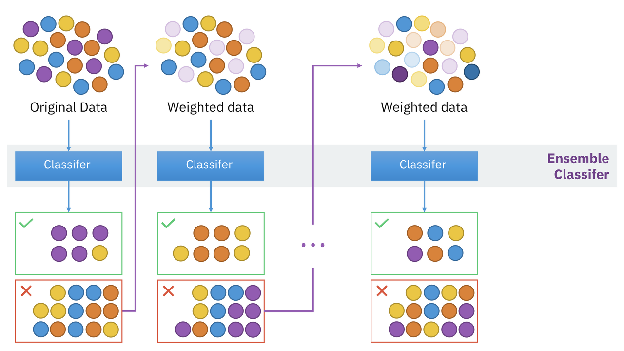
https://commons.wikimedia.org/wiki/File:Ensemble_Boosting.svg
대표적인 GBM
1. XGBoost: 병렬처리 및 근사 알고리즘을 통해 학습속도 개선
2. LightGBM: Microsoft에서 제안, 병렬 처리 없이도 빠르게 Gradient Boosting을 학습 가능
3. CatBoost: 범주형 변수에 효과적인 알고리즘을 구현하여 학습 속도 개선, 과적합 방지
'boostcamp AI Tech > 추천 시스템' 카테고리의 다른 글
| [RecSys] 추천 시스템에 Deep Learning 활용하기 2 (0) | 2023.04.03 |
|---|---|
| [RecSys] 추천 시스템에 Deep Learning 활용하기 1 (0) | 2023.04.01 |
| [RecSys] Item2Vec and ANN (0) | 2023.03.31 |
| [RecSys] 추천 시스템 - 협업 필터링 (Collaborative Filtering) - MBCF (0) | 2023.03.29 |
| [RecSys] 추천 시스템 - 협업 필터링 (Collaborative Filtering) - NBCF (0) | 2023.03.27 |